Abstract
CRISPR screens are powerful experimental tools used to screen entire genomes in search of genes responsible for phenotypes of interest. With this approach, a single experiment can generate several gigabytes of data that, with sequential implementation, can take many hours to process, limiting the depth of sequencing and amount of analysis that can feasibly be performed. Here, we apply principles of parallel computing and algorithm design to expedite the data processing and analysis pipeline significantly. In doing so, we create a framework that provides three important features: i) Facilitation of considerably deeper sequencing experiments through parallelized expedition ii) integration of a sequence distance analysis for improved screening results iii) An associated cost-performance analysis for achieving the desired computational power within given financial constraints.
Introduction
Background Information
The advent of technological advancements such as high-throughput sequencing and genome engineering, along with the increase in available computational power, has allowed biologists to adopt experimental approaches that create millions, sometimes even billions of data points per experiment. One example of such an advancement is the CRISPR genetic screen, in which researchers can introduce mutations in all twenty thousand (or so) genes in the human genome in parallel to identify new genes that are involved in a particular biological or pathological process (1).
The fundamental technology for this experimental procedure, as its name might suggest, is CRISPR genome engineering. This approach, developed from a bacterial viral defence mechanism, requires two components; a Cas9 protein, which acts like a set of molecular scissors that cuts DNA, and an RNA molecule that serves as a guide, ensuring that the Cas9 protein cuts at the specifically desired location. Using these two components, genes can be cut, copied and pasted with incredible efficiency and accuracy - and it is this efficiency that makes CRISPR genetic screens feasible.
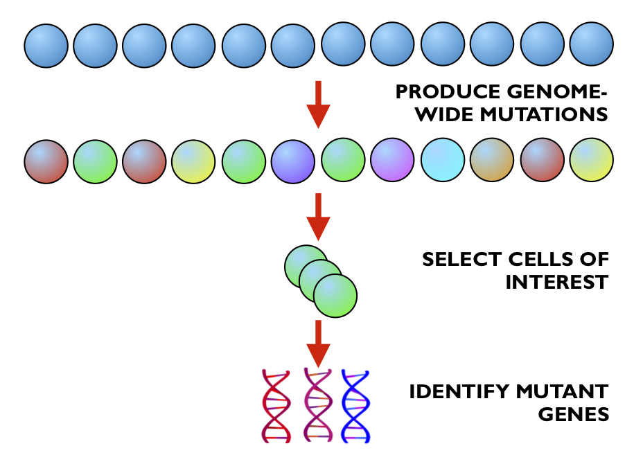
The first step of the screen is to genetically engineer your cells of interest to express the Cas9 ‘scissor’ protein, and to produce a large population of these cells. Next, you introduce a large library of different guide RNA molecules, which will stochastically insert themselves into your population of cells (with the help of some helpful little technique known as lentivirus transfection). The idea here is that every cell in your population has the potential for any of its genes to be removed (thanks to the presence of Cas9) - and through stochasticity, different cells will recieve guides and thus will cut out different genes. The result is a population of cells that have all the genes in their genomes mutated in parallel.
Once this is achieved, you select the cells that display a phenotype of interest (how exactly this is done is very dependent on the particulars of the individual experiment), and sequence the DNA to identify which genes are mutated in these cells of interest.
In our particular experimental problem, we are looking at the Shh pathway, a critical component of mammalian development. To identify cells in which this pathway is affected, the activity of this pathway is linked to the expression of a fluorescent protein, and cells with altered fluorescence are isolated with a technique known as FACS. In doing this, cells that have recieved mutations that affect this signalling pathway are identified and isolated.
Problem Description
The output of the biological experiment for a CRISPR genetic screen consists of two files of DNA sequences:
1) one file contains the DNA sequences from the control population of cells, (those that do not express the phenotype of interest) which we will call the control file
2) the second file contains the DNA sequences from cells that were selected for some phenotype of interest, which we will call the experimental file.
The goal is to identify the mutations that are enriched in the experimental file compared to the control file.
Each file generally contains ten to twelve million DNA sequences that need to be processed. Each DNA sequence must be matched to a ‘gold-standard’ reference database of ~80,000 sequences to determine its origin. This matching process involves a string-to-string comparison. Generally, about 75% of the DNA sequences in a file can be perfectly matched to the gold standard. If the DNA sequence cannot be matched perfectly to this reference database, then the edit distance between the DNA sequence and each of the 80,000 gold-standard sequences must be calculated. String-to-string edit distance calculation is a very slow process, and it takes ~36s to calculate 80,000 edit distances for a single DNA sequence. Generally, around two million input sequences do not perfectly match the database of gold-standard sequences, so calculating the edit distance between each of these sequences and the full reference database would take as much as 20,000 hours (36sec x 2M sequences / 3600 sec/hr). We would like to calculate the edit distances for the sequences that do not match any of the gold-standard sequences perfectly because this allows us to extract more information from a labor and time-intensive biological experiment.
Thus, this is a “Big Compute” problem because we need to compute these edit distances, and we are not sure which DNA sequences require edit distance calculation. Parallelization of this part of the application is required to make the application run in a reasonable amount of time (on the order of hours). Speed is also crucial because biological researchers depend on these results to execute their next experiments, which are time-sensitive because they are handling living cells and tissues.
Previous work/tools for analyzing CRISPR genetic screens includes only one published tool. MaGECK is an open-source pipeline for analyzing CRISPR screens (2) based on mean-variance modeling of the read counts for every gene. This pipeline provides read counts for genes given input control and experimental files, however it does not include an edit distance feature to determine the most likely gold-standard sequence for a sequencing read that did not perfectly match a gold-standard sequence. Additionally, MaGECK is considered a black-box program with statistics that are not well understood by general biologists. Our application would provide a missing functionality that would allow researchers to extract more information from their screens and give researchers a tool that can be clearly explained.
Existing Pipeline
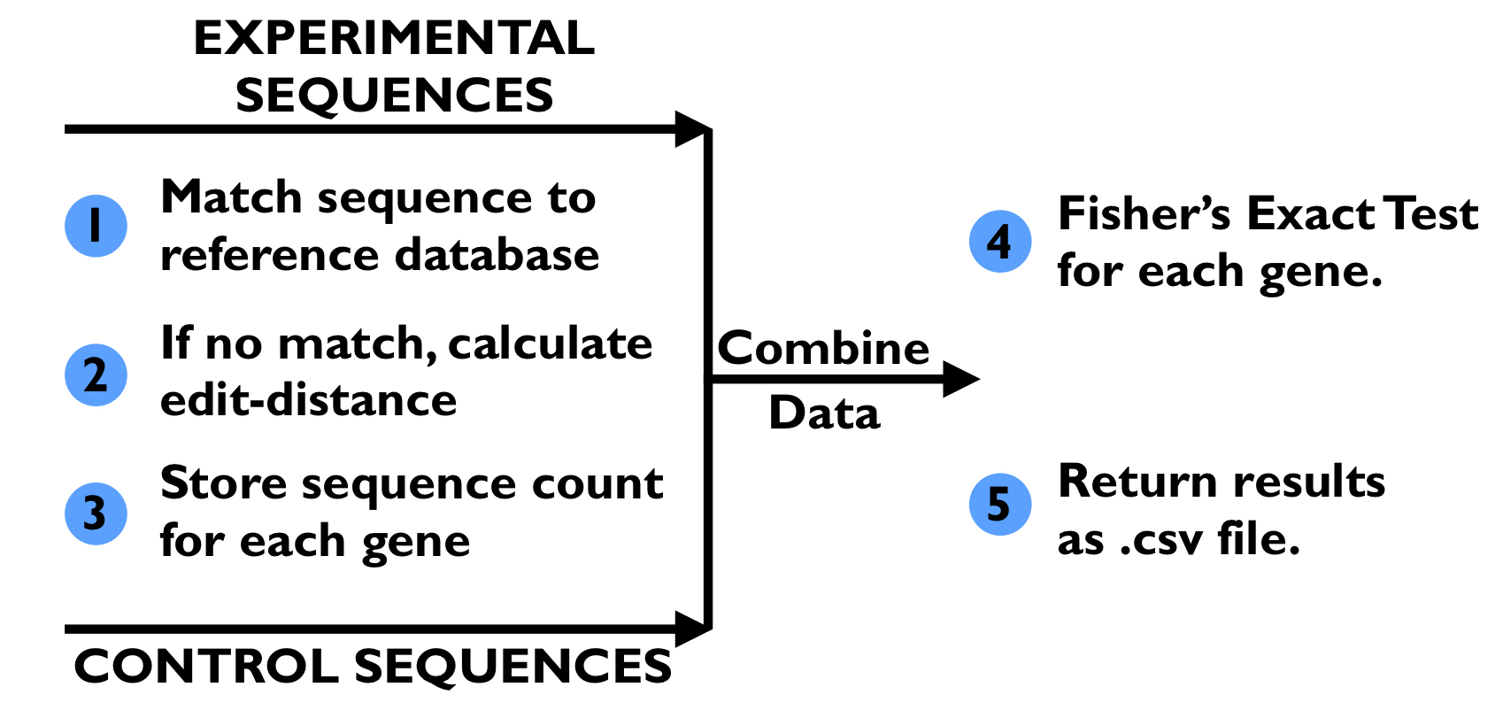 Shown above, the existing pipeline (1) takes in a control file and experiment file generated from the DNA sequencing step of the genetic screen. It also takes in a file containing the “database” of 80,000 gold-standard sequences. First, every DNA sequence in the control file is mapped to one of the gold-standard sequences; if the sequence matches one of the gold-standard sequences, then the match count for gold-standard sequence is incremented and the match count for corresponding gene is incremented. If no perfect match can be determined, then the edit distance between the control DNA sequence and every gold-standard sequence is calculated. The gold-standard DNA sequence with the lowest edit distance is found, and its match count and the match count for the corresponding gene are incremented. Once all the DNA sequences in the control file have been matched, this process is repeated for the experimental file. The match counts for genes in the control file and the experiment file are aggregated, and a Fisher’s exact test is run on the match counts from both files to determine if there is a significant change in the number of matched sequences for each gene in the experimental file when compared to the control file. The output of the pipeline consists of, for each gene, its Fisher’s exact test p-value, the number of matching sequences in the control file, the total number of sequences in the control file, the number of matching sequences in the experimental file, and the total number of sequences in the experimental file. These stats are written to a CSV file.
The code for the exisiting sequential pipeline for analyzing the results of CRISPR genetic screens can be found here. This script requires use of Python3 and relies on the use the numpy and scipy packages. Any user can install a Conda environment using the YAML file provided to run this sequential code. The Python script sequential_analysis.py takes in multiple arguments through the use of command-line flags:
1. -u indicates the file following file path if for the control file
2. -s indicates the file following file path if for the experimental file
3. -g indicates the file following file path if for a CSV file containing the 80,000 gold-standard sequences
4. -o indicates the following string will be used as a prefix for the output file
Command-line Example:
python sequential_analysis.py -u ../data/control_file_100_seqs.txt -s ../data/experimental_file_100_seqs.txt -g ../data/Brie_CRISPR_library_with_controls_guides.csv -o test_output
The output of the script is a CSV file with six columns with the following information:
1. Name of the gene
2. p-value from Fisher’s exact test for enrichment
3. Number of DNA sequences from control file mapping to gold-standard sequences contained in this gene
4. Total number of DNA sequences in control file
5. Number of DNA sequences from experimental file mapping to gold-standard sequences contained in this gene
6. Total number of DNA sequences in experimental file
An example of the output file for running the sequential analysis on the control file control_file_100_seqs.txt and the experimental file experimental_file_100_seqs.txt can be found here.
Project Design
Sequential Code Profiling
The sequential code sequential_analysis.py was profiled using the cProfile Python package. The file was run with a control file of 100 sequences (control_file_100_seqs.txt) and an experimental file of 100 sequences (experimental_file_100_seqs.txt). Each of these input files contained 75 sequencing reads that could be perfectly matched to the database of 80,000 guide sequences and 25 sequencing reads that needed an edit distance calculation. This breakdown was representative of the proportion of sequencing reads in the full input files; ~25% of sequencing reads cannot be perfectly matched to one of the 80,000 guide sequences. The exact command that was run was: python -m cProfile -o 100_seq_stats.profile sequential_analysis.py -g ../data/Brie_CRISPR_library_with_controls_FOR_ANALYSIS.csv -u ../data/Genome-Pos-3T3-Unsorted_100_seqs.txt -s ../data/Genome-Pos-3T3-Bot10_100_seqs.txt -o cProfile_test_output. This code was run on a Macbook Pro, with a 2.2 GHz Intel Core i7 processor with 6 cores. The profiling information was saved in a file called 100_seq_stats.profile. The following results are from the pstats package.
import pstats

p = pstats.Stats('100_seq_stats.profile'); #read in profiling stats
p.strip_dirs(); #remove the extraneous path from all the module names

#sort according to time spent within each function, and then print the statistics for the top 20 functions.
p.sort_stats('time').print_stats(20)
Mon Apr 29 16:08:45 2019    100_seq_stats.profile

         350132307 function calls (350126604 primitive calls) in 537.388 seconds

   Ordered by: internal time
   List reduced from 1999 to 20 due to restriction <20>

   ncalls  tottime  percall  cumtime  percall filename:lineno(function)
  3981650  462.315    0.000  534.561    0.000 count_spacers_with_ED.py:35(editDistDP)
333437825   69.985    0.000   69.985    0.000 {built-in method builtins.min}
  3982102    1.819    0.000    1.819    0.000 {built-in method numpy.zeros}
        2    1.414    0.707  535.981  267.990 count_spacers_with_ED.py:69(count_spacers)
7992171/7992125    0.447    0.000    0.447    0.000 {built-in method builtins.len}
        1    0.215    0.215    0.232    0.232 count_spacers_with_ED.py:7(createDictionaries)
    81/79    0.153    0.002    0.156    0.002 {built-in method _imp.create_dynamic}
    20674    0.115    0.000    0.365    0.000 stats.py:3055(fisher_exact)
      348    0.100    0.000    0.100    0.000 {method 'read' of '_io.FileIO' objects}
    41950    0.092    0.000    0.092    0.000 {method 'reduce' of 'numpy.ufunc' objects}
        1    0.075    0.075    0.075    0.075 {method 'dot' of 'numpy.ndarray' objects}
      348    0.056    0.000    0.155    0.000 <frozen importlib._bootstrap_external>:830(get_data)
    28062    0.052    0.000    0.052    0.000 {built-in method numpy.array}
     1604    0.035    0.000    0.035    0.000 {built-in method posix.stat}
      348    0.034    0.000    0.034    0.000 {built-in method marshal.loads}
    593/1    0.033    0.000  537.389  537.389 {built-in method builtins.exec}
        1    0.033    0.033    0.405    0.405 count_spacers_with_ED.py:135(calcGeneEnrich)
    81/65    0.024    0.000    0.077    0.001 {built-in method _imp.exec_dynamic}
    21078    0.021    0.000    0.071    0.000 fromnumeric.py:69(_wrapreduction)
    20675    0.020    0.000    0.020    0.000 {method 'writerow' of '_csv.writer' objects}
The majority of runtime is spent with editDistDP function. 534 of the 537 seconds, which accounts for 99.4% of the runtime, are spent calculating the edit distance between 50 sequencing reads and 80,000 guides. Generally, the input files contain ~10M sequencing reads, and about 25% of the sequences cannot be matched perfectly to one of the 80,000 guides. Thus for two input files of ~10M sequencing reads (~20M reads total), there are ~4-5M sequencing reads for which the edit distance calculations must be performed. If this code was run sequentially, this would require 10,000 hours of runtime. Therefore, we need to parallelize this portion of the code.
The edit distance calculation is currently nested within the function count_spacers, which matches each sequencing read from the input files to one of the 80,000 guides. For 200 sequencing reads provided as input, 1.4 seconds are spent performing the matching. This is only 0.007 seconds per sequencing read (using the 1.4 seconds from the tottime column since the cumtime takes into account the edit distance calculation). This number grows large if we have 20M sequencing reads - it would take . Thus, the entire matching process of our workflow needs to be parallelized.
Programming Model
Our application is a mix of high-throughput computing (HTC) and high-performance computing (HPC). This is an HTC job because the same task needs to be applied to every sequence in the control and experimental files; this task involves matching the sequence to one of the 80,000 gold-standard sequences and, if necessary, computing the edit distance between the sequence and each of the 80,000 gold-standard sequences. Additionally, the sequences from the input files are all independent, so they can be processed in any order. The HPC component comes from the calculation of the 80,000 edit distances for a sequence because this currently takes ~36 seconds for a single sequence, and there close to 4-5M of these sequences combined between the control and experimental files. Lastly, this is a single program, multiple data paradigm (SPMD) because the counts of all the sequences need to be aggregated for the execution of the Fisher’s exact test on each gene, so only one program can perform that task.
Code Design
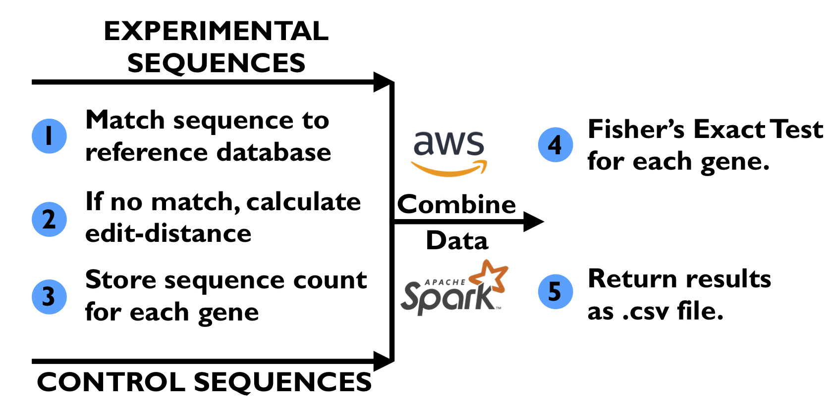
We want to parallelize this matching process by using an AWS EMR Spark cluster to have access to as many cores as possible to perform both the matching process and edit distance calculation (if needed). We will partition each input file into many tasks, and each task will run on a single core of the Spark cluster. A single core will perform both the matching process and edit distance calculation for the sequencing reads in a partition, since this would give us the best utilization of each core and instance. From what we have determined, there is not an easy way to parallelize the edit distance calculation algorithm itself, so we do not see a need for other parallelization tools such as OpenMP or MPI. Spark on AWS will be the main tool we use to parallelize this application.
The alternative approach we considered for parallelizing this application was to parallelize the calculation of the 80,000 edit distance calculations that need to be performed when a sequencing read does not perfectly match one of the gold-standard sequences. We had two ideas of how to tackle this:
- We use many instances with a large number of cores. Using Spark, we would provide a single core on a single instance with one partition. When the single core has to compute the edit distance for one of the sequencing reads, we could send this work to the other cores provided by the instance using OpenMP or Python multi-threading, thus parallelizing the 80,000 edit distance calculations. The obvious downside to this approach is that most of the cores we are paying for would be utilized only part of the time. Thus, we decided against this approach.
- We could use GPU instances in the Spark EMR cluster. Using Spark, we provide all of the CPU cores of the AWS instances with a partition to process. Whenever a CPU core has to compute the edit distance, it hands this work off to the GPU. If we try to use a GPU to perform the 80,000 edit distance calculations in parallel, memory-transfer (input/output) to the GPU would also be an added overhead. For a single sequencing read, multiple transfers would need to be performed because we would not be able to perform the 80,000 calculations completely in parallel because we are limited by the number of cores on the GPU. Additionally, use of the GPU could add extra load-balancing because for an AWS GPU instance, there are many more CPU cores than GPUs alloted to the instance. If many CPU cores need to calculate an edit distance, then there will be a queue to use the GPU(s), which prevents the CPU core from performing more sequence matching operations. Lastly, the use of GPU instances would require complex configurations to the EMR cluster, a task that is outside of our knowledge base. For these reasons, we decided not to pursue this approach either.
Scaling
The sequence matching and edit distance portion of our code accounts for 99.4% of the runtime in our small example. With larger problem sizes, this percentage should only increase because the number of operations performed after the sequence matching and edit distance section is constant.
Amdahl’s Law states that potential program speedup is defined by the fraction of code c that can be parallelized, according to the formula
where p is the number of processors/cores. In our case, c=0.994 and the table below shows the speed-ups for 2, 4, 8, 64, and 128 processors/cores:
| processors | speed-up |
|---|---|
| 2 | 1.98x |
| 4 | 3.93x |
| 8 | 7.68x |
| 64 | 46.44x |
| 128 | 72.64x |
Thus, our strong-scaling is almost linear when p is small, but we observe that this begins to break down because we only get 73x speed-up if we were to use 128 processors/cores.
Gustafson’s Law states larger systems should be used to solve larger problems because there should ideally be a fixed amount of parallel work per processor. The speed-up is calculated by
where p is the number of processors/cores. In our case, c=0.994 and the table below shows the speed-ups for 2, 4, 8, 64, and 128 processors/cores:
| processors | speed-up |
|---|---|
| 2 | 1.994x |
| 4 | 3.98x |
| 8 | 7.96x |
| 64 | 63.62x |
| 128 | 127.23x |
Thus, we almost achieve perfect weak-scaling because we can split up larger problem-sizes (which would be larger input files in our case) over more processors to achieve about the same runtime.
Edit Distance Algorithm
To calculate edit distance we applied an dynamic programming algorithm known as the Wagner-Fischer algorithm. In recognition of the fact that the vast majority of reference sequences would bare little resemblence to any particular test sequence, we implemented a speed-up heuristic that aborted the edit distance calculation for any two sequences once the edit distance grew any larger than 3. Implementing this heuristic provided a speed-up of just over 3x. The reasoning for a cut-off of 3 for edit distances is that for a sequence of 20 base-pairs, more than three differences is indicative of the sequences being poorly matched.
Infrastructure
We tested our parallelized code using m4.xlarge, m4.10xlarge, and m4.16xlarge instances.
m4.xlarge instance
The m4.xlarge instances have 4 vCPUs, 16GiB memory, and 32 GiB of EBS storage. The following information contain the architecture of the instance, the number of vCPUs, threads per core, the processor, and the cache sizes:
Architecture: x86_64
CPU(s): 4
On-line CPU(s) list: 0-3
Thread(s) per core: 2
Core(s) per socket: 2
Socket(s): 1
Model name: Intel(R) Xeon(R) CPU E5-2686 v4 @ 2.30GHz
L1d cache: 32K
L1i cache: 32K
L2 cache: 256K
L3 cache: 46080K
Additionally, m4.xlarge instances have a dedicated EBS bandwidth of 750Mbps with High network performance using the EC2 Enhanced Networking (see link).
From this information, we know that we only really have 2 cores per instance available to use, so this is the number of executor cores we will specify when using the Spark cluster.
m4.10xlarge instance
The m4.10xlarge instances have 40 vCPUs, 160GiB memory, and 32 GiB of EBS storage. The following information contain the architecture of the instance, the number of vCPUs, threads per core, the processor, and the cache sizes:
Architecture: x86_64
CPU(s): 40
On-line CPU(s) list: 0-39
Thread(s) per core: 2
Core(s) per socket: 10
Socket(s): 2
Model name: Intel(R) Xeon(R) CPU E5-2676 v3 @ 2.40GHz
L1d cache: 32K
L1i cache: 32K
L2 cache: 256K
L3 cache: 30720K
Additionally, m4.10xlarge instances have a dedicated EBS bandwidth of 4,000 Mbps with 10 Gigabit Network Performance.
From this information, we know that we only really have 20 cores per instance available to use, so this is the number of executor cores we will specify when using the Spark cluster.
m4.16xlarge instance
The m4.16xlarge instances have 64 vCPUs, 256GiB memory, and 32 GiB of EBS storage. The following information contain the architecture of the instance, the number of vCPUs, threads per core, the processor, and the cache sizes:
Architecture: x86_64
CPU(s): 64
On-line CPU(s) list: 0-63
Thread(s) per core: 2
Core(s) per socket: 16
Socket(s): 2
Model name: Intel(R) Xeon(R) CPU E5-2686 v4 @ 2.30GHz
L1d cache: 32K
L1i cache: 32K
L2 cache: 256K
L3 cache: 46080K
Additionally, m4.16xlarge instances have a dedicated EBS bandwidth of 10,000 Mbps with 25 Gigabit Network Performance.
From this information, we know that we only really have 32 cores per instance available to use, so this is the number of executor cores we will specify when using the Spark cluster.
Overheads
Since we do not know for which sequences we will need to perform edit distance calculations, load-balancing is the main overhead we anticipate dealing with because we do not want one or two cores slowed down with having to compute too many edit distance calculations. We would like to spread the number of edit distance calculations out evenly between cores by tuning the number of Spark tasks. This tuning will have to balance creating as many tasks as possible without increasing the communication and memory-management overheads Spark has to deal with when many partitions are created; we do not want the speed-up benefit of better load-balancing to get outweighed by the extra overheads due to communication and memory-management, especially when the number of instances being utilized grows very large.
Usage
Local Mode
Our Spark application can be run in local mode on a single AWS instance using the script spark_implementation_local.py. The AWS instance needs to be installed with Python3 and the packages numpy and scipy. Additionally, Apache Spark 2.2.0 must be installed.
Once those dependencies are installed, the user must execute the following command:
export PYSPARK_PYTHON=python3.x
where x is the release installed by the user.
To run the spark_implementation_local.py code using more than one core on a single instance, the user can modify the spark_implementation.py code by including a [c] (where c=2 or greater) in the code at SparkConf().setMaster('local[c]').
spark_implementation_local.py takes in multiple arguments through the use of command-line flags:
1. -u indicates the file following file path if for the control file
2. -s indicates the file following file path if for the experimental file
3. -g indicates the file following file path if for a CSV file containing the 80,000 gold-standard sequences
4. -o indicates the following string will be used as a prefix for the output file
The following command is an example of how to run the application in local mode:
spark-submit spark_implementation_local.py -u control_file_100_seqs.txt -s experimental_file_100_seqs.txt -g Brie_CRISPR_library_with_control_guides.csv -o spark_run_1_core.
Distributed Mode
Our Spark application can be run in distributed mode on an AWS EMR Spark cluster using the script spark_implementation_distributed.py. We used “emr-5.8.0” when creating clusters for our tests. AWS EMR Spark clusters already come with Python3.4, numpy and scipy installed. Before running the application, the user must execute the following command:
export PYSPARK_PYTHON=python3.4
.
spark_implementation_distributed.py takes in multiple arguments through the use of command-line flags:
1. -u indicates the file following file path if for the control file
2. -s indicates the file following file path if for the experimental file
3. -g indicates the file following file path if for a CSV file containing the 80,000 gold-standard sequences
4. -o indicates the following string will be used as a prefix for the output file
5. -n indicates the number of partitions that the control and experimental file should be split into to be processed on the cluster
This Spark application conveniently takes care of placing the control file and experimental file into the Hadoop file system, so the user does not need to do this prior to running the application.
The following command is an example of how to run the application in distributed mode:
spark-submit --num-executors 2 --executor-cores 2 spark_implementation_distributed.py -u control_file_100_seqs.txt -s experimental_file_100_seqs.txt -g Brie_CRISPR_library_with_control_guides.csv -o spark_distrb_output -n 50
Results
Data
We used two pairs of datasets to evaluate our code. These datasets were derived from DNA sequencing files from an original CRISPR genetic screen (1). Sequences for the control file are taken from a larger control dataset, while sequences for the experimental file are taken from a larger experimental dataset.
The first dataset consists of two a control file of 100 sequences (control_file_100_seqs.txt) and an experimental file of 100 sequences (experimental_file_100_seqs.txt). As explained earlier, each of these input files contains 75 sequencing reads that could be perfectly matched to the database of 80,000 guide sequences and 25 sequencing reads that needed an edit distance calculation. This breakdown is representative of the proportion of sequencing reads in the full input files because ~25% of sequencing reads cannot be perfectly matched to one of the 80,000 guide sequences.
The second dataset used for evaluation is 10x larger than the previous dataset. This dataset consists of a a control file of 1000 sequences (control_file_1000_seqs.txt) and an experimental file of 100 sequences (experimental_file_1000_seqs.txt). These two files were also constructed so that each one contains 750 sequencing reads that can perfectly matched to one of the 80,000 guides and 250 sequences that require an edit distance calculation. This second dataset was used to evaluate how Spark clusters of more powerful instances perform.
Testing Sequential Code on Single m4.xlarge Instance
To ensure the fidelity of our sequential code on AWS, we ran it on a single m4.xlarge instance with the control_file_100_seqs.txt and experimental_file_100_seqs.txt as input files. We used the command
python3 sequential_analysis.py -g Brie_CRISPR_library_with_controls_FOR_ANALYSIS.csv -u control_file_100_seqs.txt -s experimental_file_100_seqs.txt -o output_seq
.
This test took 12 minutes and 54 seconds to run sequentially and the output file matched the output file when the sequential code was run on a MacBook Pro.
Testing Spark Code in Local Mode on Single m4.xlarge Instance
The code for this is available here.
This Spark application was run on the testing input files control_file_100_seqs.txt and experimental_file_100_seqs.txt. It was run with only 1 or 2 cores were tried, because AWS only allots two physical cores per m4.xlarge instance. We modified the spark_implementation_local.py code by including a [c] (where c=2) in the code at SparkConf().setMaster('local[c]').
The following command was used to run tests:
spark-submit spark_implementation_local.py -u control_file_100_seqs.txt -s experimental_file_100_seqs.txt -g Brie_CRISPR_library_with_control_guides.csv -o spark_run_1_core.
The table below lists the number of cores used in local mode, the elapsed time, and the speed-up.
| Number of cores | Elapsed time | Speed-up |
|---|---|---|
| 1 | 685 sec | - |
| 2 | 352 sec | 1.94x |
This test of the Spark code on a single core of the m4.xlarge instance will be the baseline. All of the speed-ups below will be calculated based on this performance.
Testing Spark Code on Cluster of m4.xlarge Instances
The code for this is available here.
To tune the task/partition value for breaking up the input files, the Spark application was changed to be able to take in a user-defined variable for the number of partitions the input files should be split into through command-line; the flag -n allows the user to define the number of partitions. Within this code, the partition number for Spark was changed by adding an argument in sc.textFile("control_file_100_seqs.txt", n) where n is the number of partitions specified by the user through the -n flag.
The table below shows efforts to tune different parameters and improve the speed-up when using up to 8 nodes. The speed-up is compared to the performance of 1 core on 1 node of a m4.xlarge instances.
The following command was used to generate the stats in the table:
spark-submit --num-executors 2 --executor-cores 2 spark_implementation_distributed.py -u control_file_100_seqs.txt -s experimental_file_100_seqs.txt -g Brie_CRISPR_library_with_control_guides.csv -o spark_run_4_core -n 4
Parameters were varied as seen in the table below.
| Number of worker nodes | Number of cores | Number of tasks | Elapsed time | Speed-up |
|---|---|---|---|---|
| 2 | 2 | 4 | 439 sec | 1.56x |
| 2 | 2 | 32 | 249 sec | 2.75x |
| 2 | 2 | 50 | 243 sec | 2.82x |
| 4 | 2 | 32 | 144 sec | 4.76x |
| 4 | 2 | 50 | 148 sec | 4.63x |
| 8 | 2 | 32 | 139 sec | 4.93x |
| 8 | 2 | 50 | 81 sec | 8.46x |
| 8 | 2 | 75 | 106 sec | 6.46x |
Only two cores per worker node were specified for these experiments because even though AWS says m4.xlarge instance have 4 vCPUs, AWS only allots 2 physical cores to these instances.
From this table, we see that more cores and more tasks give better performance. Interestingly, with 8 nodes and using 2 cores on each node, for a total of 16 threads, the performance is about equivalent to using 4 instances with 2 cores each. This is most likely because the 32 tasks on the 8 nodes causes load-balancing issues where one or two nodes get slowed down by too many edit distance calculations. Once we increase the number of tasks/partitions to 50, we see that we get ~8.5x speed-up. For these input files of 100 sequencing reads each, 75 tasks/partitions introduces more synchronization and communication overhead for Spark resulting in lower performance than the run with 50 tasks.
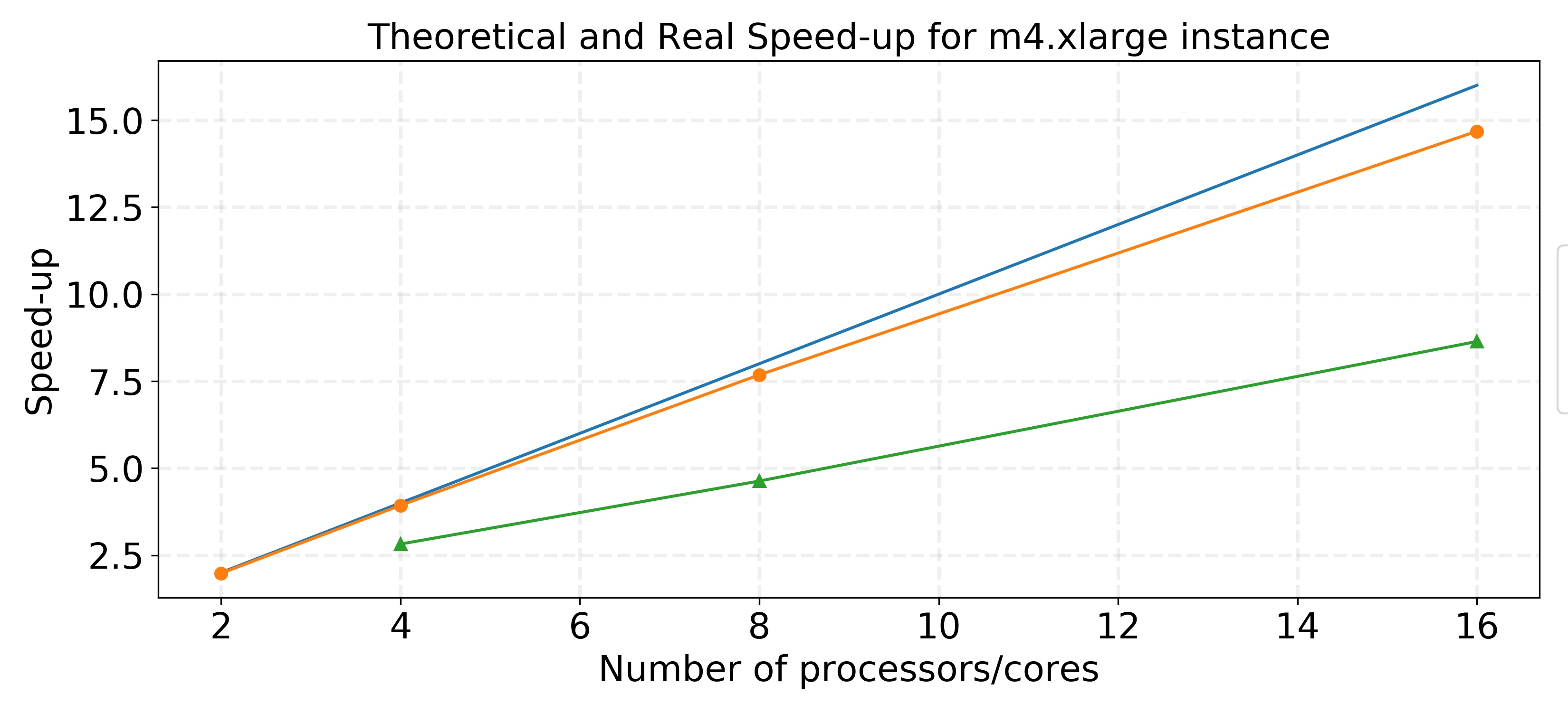 The speedup plot in this graph is based on the performances using 50 partitions/tasks. The blue line represents linear speed-up, the orange line represents the theoretical speed-up according to Amdahl’s Law, and the green line is the real, observed speed-up.
The real speed-up achieved is lower than the theoretical speed-up calculated using Amdahl’s Law for a fixed problem size. As we increase the number of processors, the real speed-up does not follow the close-to-linear trend that was theoretically calculated. This is likely due to increased overhead due to data management and movement caused by using more cores and smaller partitions.
Since we do not know which sequences from our input files we will need to perform edit distance calculations for, it is probably best to separate the input file into as many partitions as possible because this will spread out the sequences that require edit distance calculations over as many cores as possible. As seen above and talked about in the Overheads section, there is a performance-overhead trade-off when using more and more partitions. Using a few instances with many cores may prove to be better than using many instances that each have a couple of cores.
Next, we scaled up the problem size and instance size.
Testing with Input Files containing 1000 sequences
We scaled up the input files ten-fold by making each input file 1000 sequence reads, as described in the Data section. Even using two 1000 sequence read files is only $0.01$% of our full dataset.
If we were to run these input files on a single m4.xlarge instance using 1 core, we calculate that this would take
Below is a table of the performance of multiple m4.xlarge instances on these 1000 sequence input files. The speed-up is calculated against our calculation of how long it would take to process this data on one core of a m4.xlarge instance.
| Number of worker nodes | Number of cores | Number of tasks | Elapsed time | Speed-up |
|---|---|---|---|---|
| 8 | 2 | 50 | 699 sec | 9.79x |
| 8 | 2 | 100 | 634 sec | 10.8x |
| 8 | 2 | 500 | 600 sec | 11.4x |
Even with scaling up the problem size, we see that we can achieve very good speed-up by tuning the number of partitions.
Testing with m4.10xlarge Instances in Cluster
We now scaled up the instance types by creating a Spark cluster of m4.10xlarge instances, which each have 20 physical cores alloted to them. We had asked AWS for at least 9 m4.10xlarge so we could use 8 worker nodes, however AWS denied this request due to our lack of usage and their resource constraints. A compromise was made at 5 instances. Thus, we created a Spark cluster of 1 master node and 4 worker nodes.
The following command was run to test the 1000 sequence input files on this cluster:
spark-submit --num-executors 4 --executor-cores 20 spark_implementation_distributed.py -u control_file_1000_seqs.txt -s experimental_file_1000_seqs.txt -g Brie_CRISPR_library_with_control_guides.csv -o spark_run_m410 -n 250.
Parameters were varied as seen in the table below.
The speed-up is calculated against our calculation of how long it would take to process this data on one core of a m4.xlarge instance.
| Number of worker nodes | Number of cores | Number of tasks | Elapsed time | Speed-up |
|---|---|---|---|---|
| 2 | 20 | 500 | 277 sec | 24.7x |
| 4 | 20 | 250 | 191 sec | 35.9x |
| 4 | 40 | 250 | 185 sec | 37x |
| 4 | 20 | 500 | 160 sec | 42.8x |
| 4 | 20 | 750 | 159 sec | 43.1x |
To ensure that the using 20 cores per instance is correct, we also did a test with 40 cores per instance. Even though the m4.10xlarge instances offer 40 vCPUs, the speed-up by specifying 20 cores versus 40 cores when using 250 tasks is not very different, indicating that the user is really only getting 20 threads/cores.
500 tasks/partitions for these files of 1000 sequences seems optimal since there is noticeable performance improvement from 250 tasks to 500 tasks and little improvement from 500 tasks to 750 tasks. We also observe that there is some increase in the overhead when using more instances/nodes because the speed-up does not scale linearly as we increase the number of total cores used. When the number of tasks is kept constant (n=500), we get a speed-up of 24.7x with 40 total cores, so in a perfect world, we would get a speed-up of ~49x with 80 cores. However, we only get a speed up of 42.8x when we use 80 total cores. There must be an increase in communication and memory management that Spark has to deal with when more cores are used, which is expected.
Testing with m4.16xlarge Instances in Cluster
Lastly, we scaled up the instance types by creating a Spark cluster of m4.16xlarge instances, which each have 32 physical cores alloted to them. We had asked AWS for at least 9 m4.16xlarge so we could use 8 worker nodes, however AWS denied this request due to our lack of usage and their resource constraints. A compromise was made at 5 instances. Thus, we created a Spark cluster of 1 master node and 4 worker nodes.
The following command was run:
spark-submit --num-executors 4 --executor-cores 32 spark_implementation_distributed.py -u control_file_1000_seqs.txt -s experimental_file_1000_seqs.txt -g Brie_CRISPR_library_with_control_guides.csv -o spark_run_m416 -n 250.
Parameters were varied as seen in the table below.
The speed-up is calculated against our calculation of how long it would take to process this data on one core of a m4.xlarge instance.
| Number of worker nodes | Number of cores | Number of tasks | Elapsed time | Speed-up |
|---|---|---|---|---|
| 2 | 32 | 500 | 195 sec | 35.1x |
| 4 | 32 | 250 | 156 sec | 43.9x |
| 4 | 64 | 250 | 150 sec | 45.7x |
| 4 | 32 | 500 | 129 sec | 53.1x |
| 4 | 32 | 750 | 123 sec | 55.7x |
As we did with the m4.10xlarge cluster, we made sure that 32 cores was the right number to specify for the number of cores per node by testing the performance of both 32 cores/node and 64 cores/node. AWS says that a m4.16xlarge instance has 64 vCPUs, however again we see that there is very little difference in the performance between specifying 32 cores/node and 64 core/node. Thus, we did the rest of our tests with 32 core/node.
Again, we observe that 500 tasks seem optimal for this problem size of 1000 sequences per input file, even with the availability of more cores. Like with the m4.10xlarge instances, we also see that there is some increased overhead when we increase the number of total cores used from 64 to 128 (fixed number of partitions at 500) because with 128 cores we should be able to achieve ~70x speed-up, but we only see 53x speed-up.
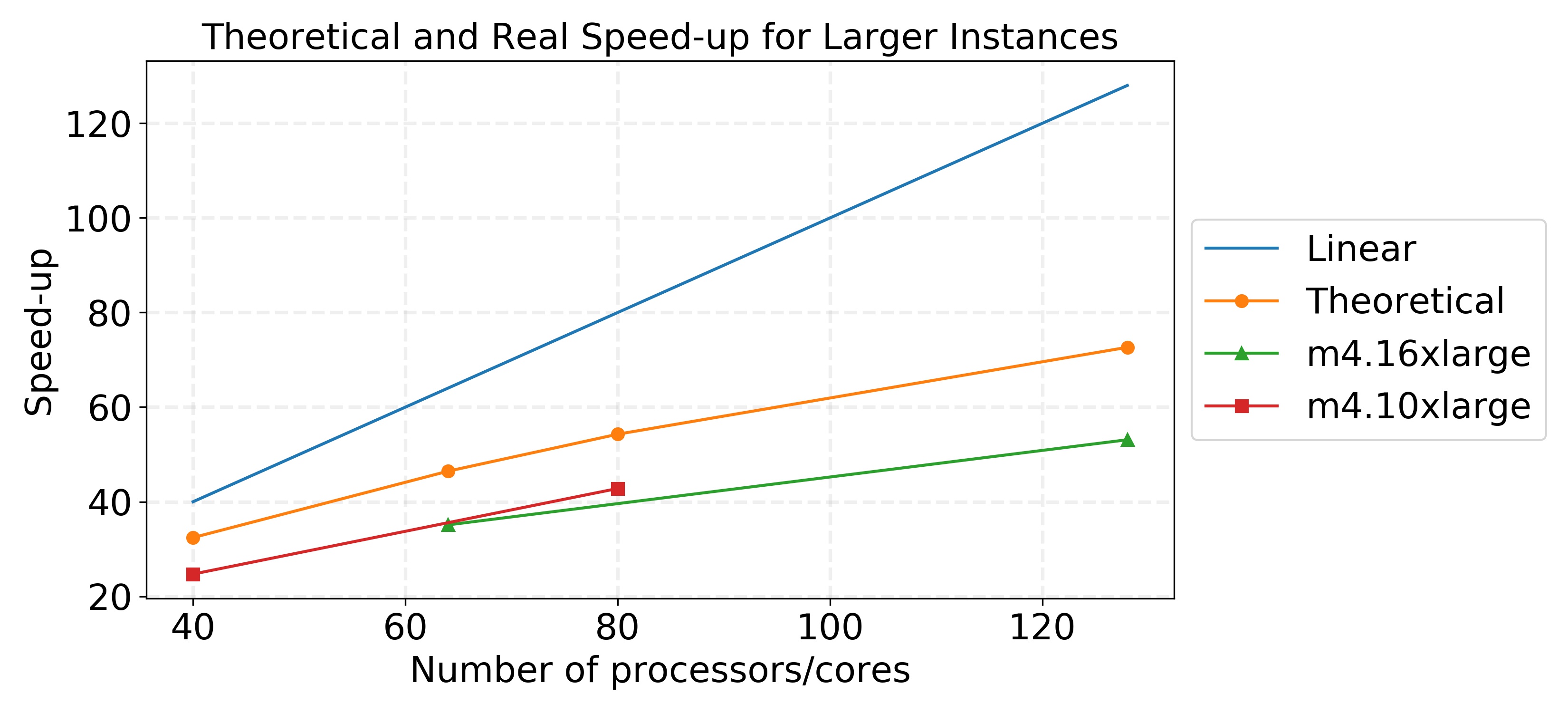 The speed-up used for the m4.10xlarge and m4.16xlarge instances in the graphs are based on using 500 tasks/partitions. Although 99% of our runtime for this application comes from a portion of the code that is parallelized, we see that our theoretical speed-up falls quite far under the linear speed-up we would hope to achieve. However, our true speed-up is even below the theoretical speed-up, as we observed for the m4.xlarge instances, because there are increases in communication and memory management overheads as more instances and cores are used. It is important to acknowledge these overheads because sometimes they can be mitigated but usually never eliminated.
Extrapolation to full dataset
To fully analyze a CRISPR genetic screen, ~20M sequences need to be processed. About 4-5M of these sequences require edit distance calculations. Using our best results with 4 m4.16xlarge instances and 32 cores/node, it takes
1,290,000 seconds is ~15 days to get the results of the genetic screen. When this is compared to the sequential runtime of ~833 days (sequential pipeline takes about 20,000 hours to run), this is quite the improvement in performance. Although 15 days is still too long for the biologists to wait for this analysis, this application demonstrates that this process can be improved immensely. Adding more instances to the cluster and trying other instances with greater number of cores, such as the m5.24xlarge (48 physical cores), would further decrease the runtime (this instance is not supported by emr-5.8.0 so we did not try it).
Cost-Performance Analysis
As an advanced feature of our application, we performed a cost-performance analysis to determine the optimal instance type to use for executing our application.
We extrapolate the improvements in runtime based on improvements made with fewer instances and cores. AWS wouldn’t allow us to provision enough instances that would allow us to test these extrapolations. However we only extrapolated performance tested on 2-4 instances to up to 15 instances, and so although clusters of a larger size would have more overhead (and hence lower performance than we anticipate), we felt comfortable using these assumptions.
We found that each of our instances had different optimal use models that relied on the number of instances provisioned. Because runtime and cost have non-linear relationships with number of instances (runtime is roughly inversely proportional to the number of instances provisioned), depending on the performance profile desired (i.e. runtime in a matter of days or weeks), different instances might be recommended to the user.
In particular - we found that using an EMR cluster consisting of larger instances (either m4.10xlarge or m4.16xlarge) was more efficient that using a cluster of smaller instances (m4.xlarge). Intuitively this makes sense since the overhead associated with multiple cores within an instance will be lower than the overhead associated with multiple cores amongst different instances. We found that for a user seeking to save money, running our program on a few m4.16xlarge instances made sense (although the code would take close to a month to run), but if speed was of the essence, using a large cluster of m4.10xlarge instances would prove to be more efficient. This is perhaps because of the fact that for this instance (with 20 cores), a balance is being struck between the communication overheads within and amongst the cores on different instances.
Overall we believe that this cost vs. performance profile will prove to be useful to potential users, helping them determine which infrastructure model to use based on their needs and budget.

Discussion
Goals and Improvement
Our goal for this project was to build an application that parallelized the mapping and edit distance operations of the analysis pipeline. We successfully built this application using Spark and achieved very good speed-up. However, this application still is not ideal for the timeline on which biologists performing CRISPR genetic screens would like to have their results because by our calculation, the runtime on a full dataset would take ~15 days based on our tests. We believe that with access to a greater number of instances and resources this performance could increase greatly, but those tests would need to be run in the future.
Based on our cost-performance analysis for using AWS instances for running this application, we observe costs in the thousands of dollars, which may not be feasible for biologists’ budgets. First, it would be worth testing the performance of our application on a cluster of c4.8xlarge instances because these instances have 18 physical cores dedicated to them (2 less cores than the m4.10xlarge instances) and only cost $1.59 per hour, which is ~$0.40 cheaper than a m4.10xlarge instance. It is possible this instance could provide a better cost-performance trade-off. Second, because of the explosion of “Big Data” in biology, many research institutions have created their own high-performance computings clusters, such as Harvard’s Odyssey and Stanford’s Sherlock clusters. Using the computing resources of these clusters would probably be ideal for this application since we need access to as many cores as possible based on the way the application is currently built.
Challenges and Lessons Learnt
One of the main challenges that we ran into was gaining access to high-performance computing instances on AWS. We were unable to get our instance limits for the m4.10xlarge and m4.16xlarge to the desired number since we were still “novices” in using AWS services. It would have been interesting to test our application on clusters of 8, 16 and even 32 worker nodes, so we could better understand our performance and scaling. Furthermore, we thought this application would be something that a user could download and use on his/her own AWS cluster. However, it would probably be very difficult for a novice AWS user (as we assume most biologists are) to get a hold of large number of HPC instances needed to use this application. Thus, this application would ideally have to be hosted some through some system.
Another challenge we ran into was that parallelizing through a Spark cluster makes it difficult to use other programming models that we learned. AWS clusters can be initialized with certain software (like OpenACC or OpenMP) using bootstrapping, however this was something we could not figure out, which limited the solution we developed. Furthermore, these clusters must be initiated with every use, which can require some waiting (sometimes 30-40min depending on instance type), and shutdown after every use. This is another reason that using a HPC cluster could be ideal. Future work would focus on integrating the other programming models with Spark to produce a more efficient pipeline that could perform the task we desire in a reasonable time.
Future Work
- Allow user to specify where input files are in an S3 bucket. Currently, this would require more configuration in the Spark application to take in a user’s private key in addition to the path to the input files, thus we did not implement this now.
- Test the use of GPUs for calculating edit distance 80,000 times for a sequence. Due to the difficulty of configuring a Spark cluster to run with GPU instances (installation of CUDA and OpenACC on each worker node), we did not try to implement this. This would require extra overhead as well because of memory movement to/from GPU; NVIDIA Tesla K80 has about 5000 cores, so we would have to perform at least 16 read and write operations to/from GPU memory to calculate the edit distances for a single sequence.
- Analyze control and experimental files on separate clusters and use some message passing to synchronize the processes. It would be interesting to try this form of parallelization, since it would cut the runtime in half because the control and experimental files are usually the same size. This form of parallelization could get very expensive for the user however.
References
- Pusapati GV, Kong JH, Patel BB, Krishnan A, Sagner A,
Kinnebrew M, Briscoe J, Aravind L, Rohatgi R: CRISPR screens
uncover genes that regulate target cell sensitivity to the
morphogen sonic hedgehog. Dev Cell 2018, 44:113-129 e118.
- Li, W., Xu, H., Xiao, T., Cong, L., Love, M.I., Zhang, F., Irizarry, R.A., Liu, J.S., Brown, M., and Liu, X.S. (2014). MAGeCK enables robust identification of essential genes from genome-scale CRISPR/Cas9 knockout screens. Genome Biol. 15, 554.